Difference between revisions of "Birds Eye View/Introduction/Research"
m |
|||
| (7 intermediate revisions by 3 users not shown) | |||
| Line 1: | Line 1: | ||
<noinclude> | <noinclude> | ||
| − | {{Birds Eye View/Head|next= | + | {{Birds Eye View/Head|next=Introduction/Dataset|previous=Introduction|keywords=|title=RidgeRun's Birds Eye View project research }} |
</noinclude> | </noinclude> | ||
| Line 7: | Line 7: | ||
--> | --> | ||
| − | = Introduction = | + | == Introduction == |
| − | |||
| − | |||
| + | In general, the camera-on-vehicle has a serious perspective effect as Fig. 1(a). Because of the perspective effect, the driver can’t feel distance correctly and advanced image processing or analysis becomes difficult also. Consequently, as Fig. 1(b), perspective transformation is necessary. The raw images have to be transferred into bird’s-eye view as Fig. 1(c). [https://www.researchgate.net/profile/Kyeong_yuk_Min/publication/224117777_Low-cost_implementation_of_bird's-eye_view_system_for_camera-on-vehicle/links/0c9605310500039383000000/Low-cost-implementation-of-birds-eye-view-system-for-camera-on-vehicle.pdf] | ||
| + | <br> | ||
[[File:PerspectiveBEV.png|600px|center|thumb| Illustration of perspective transformation in a parking lot scene [https://www.researchgate.net/profile/Kyeong_yuk_Min/publication/224117777_Low-cost_implementation_of_bird's-eye_view_system_for_camera-on-vehicle/links/0c9605310500039383000000/Low-cost-implementation-of-birds-eye-view-system-for-camera-on-vehicle.pdf]]] | [[File:PerspectiveBEV.png|600px|center|thumb| Illustration of perspective transformation in a parking lot scene [https://www.researchgate.net/profile/Kyeong_yuk_Min/publication/224117777_Low-cost_implementation_of_bird's-eye_view_system_for_camera-on-vehicle/links/0c9605310500039383000000/Low-cost-implementation-of-birds-eye-view-system-for-camera-on-vehicle.pdf]]] | ||
| − | + | <br> | |
| − | To obtain the output bird-s eye view image a transformation using the following projection matrix can be used. It maps the relationship between pixel (x,y) of bird's eye view image and pixel (u,v) from the input image. | + | To obtain the output bird-s eye view image a transformation using the following projection matrix can be used. It maps the relationship between pixel (x,y) of the bird's eye view image and pixel (u,v) from the input image. |
<center> | <center> | ||
| Line 39: | Line 39: | ||
</center> | </center> | ||
| − | The transformation is usually referred as Inverse Perspective Mapping (IPM) [http://cvrs.whu.edu.cn/downloads/ebooks/Multiple%20View%20Geometry%20in%20Computer%20Vision%20(Second%20Edition).pdf]. IPM takes as input the frontal view, applies a homography and creates a top-down view of the captured scene by mapping pixels to a 2D frame (Bird's eye view). | + | The transformation is usually referred to as Inverse Perspective Mapping (IPM) [http://cvrs.whu.edu.cn/downloads/ebooks/Multiple%20View%20Geometry%20in%20Computer%20Vision%20(Second%20Edition).pdf]. IPM takes as input the frontal view, applies a homography, and creates a top-down view of the captured scene by mapping pixels to a 2D frame (Bird's eye view). |
| − | In practice, IPM works great in the immediate proximity of car, for example, and assuming the road surface is planar. Geometric properties of objects in the distance are affected unnaturally by this non-homogeneous mapping, as shown in Figure 2 left image. This limits the | + | In practice, IPM works great in the immediate proximity of a car, for example, and assuming the road surface is planar. Geometric properties of objects in the distance are affected unnaturally by this non-homogeneous mapping, as shown in Figure 2 left image. This limits the performance of applications in terms of accuracy and distance where they can be applied reliably. The right image can be achieved by applying several post-transformation techniques like Incremental Spatial Transformer [https://arxiv.org/pdf/1812.00913.pdf]. However, this project uses a basic IPM approach as a demonstration. |
| − | There are 3 assumptions when working without post transformation techniques: | + | There are 3 assumptions when working without post-transformation techniques: |
#The camera is in a fixed position with respect to the road. | #The camera is in a fixed position with respect to the road. | ||
#The road surface is planar. | #The road surface is planar. | ||
#The road surface is free of obstacles. | #The road surface is free of obstacles. | ||
| − | = RidgeRun BEV Demo Workflow = | + | == Camera Model and Homography == |
| + | |||
| + | From the point of view of geometriacal characteristics, a pin-hole camera is a device that transforms a 3D world coordinate into a 2D image coordinate. This relation is described by the homography equation [http://www.cc.kyoto-su.ac.jp/~kano/pdf/paper/2008%20IEICE%20Top%20View.pdf]: | ||
| + | |||
| + | <center> | ||
| + | <math> | ||
| + | [u,v,1]^t \simeq P_{3x4} \cdot [X,Y,Z,1]^t \;\;\;\;\;\; (1) | ||
| + | </math> | ||
| + | </center> | ||
| + | |||
| + | Matrix is decomposed into: | ||
| + | <center> | ||
| + | <math> | ||
| + | P_{3x4} = K_{3x3} \cdot [R_{3x3}|t_{3x1}] \;\;\;\;\;\; (2) | ||
| + | </math> | ||
| + | </center> | ||
| + | |||
| + | Where <math display="inline"> R_{3x3} </math> is a 3x3 rotation matrix, <math display="inline"> t_{3x1} </math> is a 3x1 translation vector, and <math display="inline">[R_{3x3}|t_{3x1}] </math> is a 3x4 matrix reflecting the concatenation of previous two, which handles the camera position and angles relative to the 3D world coordinate frame. | ||
| + | |||
| + | The homogeneous 3D coordinate of the point on the plane is described by (3), where <math display="inline"> Q </math> is a 4x3 matrix. | ||
| + | |||
| + | <center> | ||
| + | <math> | ||
| + | [X,Y,Z,1]^t = | ||
| + | \begin{bmatrix} | ||
| + | x \cdot i + y \cdot j + d \\ | ||
| + | 1 | ||
| + | \end{bmatrix} | ||
| + | = Q_{4x3} \cdot [x,y,1]^t | ||
| + | \;\;\;\;\;\; (3) | ||
| + | </math> | ||
| + | </center> | ||
| + | |||
| + | By substituting (3) for (1), (4) is obtained which indicates the relation between the 2D coordinates of a plane in the scene and the image plane is described by a 3x3 matrix H in the homogeneous sense. | ||
| + | |||
| + | <center> | ||
| + | <math> | ||
| + | [u,v,1]^t \simeq P_{3x4} \cdot Q_{4x3} \cdot [x,y,1]^t | ||
| + | = H_{3x3} \cdot [x,y,1]^t | ||
| + | \;\;\;\;\;\; (4) | ||
| + | </math> | ||
| + | </center> | ||
| + | |||
| + | == RidgeRun BEV Demo Workflow == | ||
The following image shows the basic processing path used by the BEV system. | The following image shows the basic processing path used by the BEV system. | ||
| − | #'''Capture camera frames:''' Obtain frames from video source. 4 cameras with 180 degrees view angle. | + | #'''Capture camera frames:''' Obtain frames from a video source. 4 cameras with 180 degrees view angle. |
#'''Resize frames:''' Resize input frames to desired input size. | #'''Resize frames:''' Resize input frames to desired input size. | ||
#'''Remove lens distortion:''' Apply lens undistortion algorithm to remove the fisheye effect. | #'''Remove lens distortion:''' Apply lens undistortion algorithm to remove the fisheye effect. | ||
| Line 58: | Line 101: | ||
##'''Perspective mapping:''' Map the points from the front view image to a 2D top image (BEV) | ##'''Perspective mapping:''' Map the points from the front view image to a 2D top image (BEV) | ||
##'''Enlarging:''' Enlarge the image to search for the required region of interest (ROI) | ##'''Enlarging:''' Enlarge the image to search for the required region of interest (ROI) | ||
| − | ##'''Cropping:''' Crop the output of enlargement process to adjust the needed view. | + | ##'''Cropping:''' Crop the output of the enlargement process to adjust the needed view. |
#'''Create a final top view image''' | #'''Create a final top view image''' | ||
| Line 65: | Line 108: | ||
[[File:Transformation BEW.png|800px|center|thumb| Perspective transformation internal workflow]] | [[File:Transformation BEW.png|800px|center|thumb| Perspective transformation internal workflow]] | ||
| − | = Removing fisheye distortion = | + | == Removing fisheye distortion == |
| − | Wide angle cameras are needed to obtain the max point of view and to achieve the Bird's Eye View perspective. Usually these cameras provide fish eye image which needs to be | + | Wide-angle cameras are needed to obtain the max point of view and to achieve the Bird's Eye View perspective. Usually, these cameras provide fish eye image which needs to be transformed to remove the distortion. |
After the camera calibration process was done, done parameters are received: | After the camera calibration process was done, done parameters are received: | ||
| Line 148: | Line 191: | ||
</center> | </center> | ||
| − | = Perspective Mapping = | + | == Perspective Mapping == |
| − | The first step is to apply the perspective mapping from the input image to transform the angle image into a top view. Then, the enlarge process allows | + | The first step is to apply the perspective mapping from the input image to transform the angle image into a top view. Then, the enlarge process allows matching the output image perspective and the crop step handles to capture the required region of interest, as seen in the following image. |
<center> | <center> | ||
[[File:BEV Steps Example.png|center|900px|thumb|BEV Steps Example ]] | [[File:BEV Steps Example.png|center|900px|thumb|BEV Steps Example ]] | ||
</center> | </center> | ||
| + | == Process Optimization == | ||
| + | |||
| + | The process described so far is based on state-of-the-art papers and research on how to apply IPM and other techniques to generate a top view image. The minimal steps always include the perspective mapping to get the IPM result, enlargement to adjust the measures between different cameras, and cropping to use only the required part of the image. These steps work great for a single image in an isolated environment to analyze and generate a single output frame. However, when the process needs to be repeated once for each frame at higher frame rates the system stress might be too high, and therefore the frame rate might be lower than expected. | ||
| + | |||
| + | To enhance the performance of the library we designed a simple method to wrap up all of the steps in a single warp perspective method. Usually, in Computer Vision, two images of the same planar surface in space can be related by a homography matrix. The method has many practical applications like image rectification, image registration, or computation of camera motion rotation, resize, and translation between two images. We will rely on the last application to speed up the process. | ||
| + | |||
| + | <br> | ||
| + | <center> | ||
| + | <math> | ||
| + | H = \begin{bmatrix} | ||
| + | h_{00} & h_{01} & h_{02}\\ | ||
| + | h_{10} & h_{11} & h_{12}\\ | ||
| + | h_{20} & h_{21} & h_{22} | ||
| + | \end{bmatrix} | ||
| + | </math> | ||
| + | </center> | ||
| + | |||
| + | From an input image we need to map each <math display="inline">x_1,y_1</math> source point to another <math display="inline">x_2,y_2</math> destination point. The library uses a chessboard to collect inner corners and automatically adjust them by generating a perfect squared relationship and generate the output image as seen in the following figure. | ||
| + | |||
| + | [[File:BEV OptimizedProcess.png|900px|frameless|center]] | ||
| + | |||
| + | The relationship between the points is defined by: | ||
| + | |||
| + | <br> | ||
| + | <center> | ||
| + | <math> | ||
| + | \begin{bmatrix} | ||
| + | x_{1} \\ | ||
| + | y_{1} \\ | ||
| + | 1 | ||
| + | \end{bmatrix} = | ||
| + | |||
| + | H \cdot | ||
| + | \begin{bmatrix} | ||
| + | x_{2} \\ | ||
| + | y_{2} \\ | ||
| + | 1 | ||
| + | \end{bmatrix} = | ||
| + | |||
| + | \begin{bmatrix} | ||
| + | h_{00} & h_{01} & h_{02}\\ | ||
| + | h_{10} & h_{11} & h_{12}\\ | ||
| + | h_{20} & h_{21} & h_{22} | ||
| + | \end{bmatrix} | ||
| + | \begin{bmatrix} | ||
| + | x_{2} \\ | ||
| + | y_{2} \\ | ||
| + | 1 | ||
| + | \end{bmatrix} | ||
| + | </math> | ||
| + | </center> | ||
| + | |||
| + | The main objective is to focus on how to adjust the homography matrix to absorb all the previous steps. With several geometric transformation the library also allows the user to fine-tune the final image. Matrix multiplication allows the quick and easy modification of the final homography, therefore the operation will be defined by <math display="inline">T_1</math> (Move image to origin), <math display="inline">S_1</math> (Scale image), <math display="inline">T_2</math> (Move image back to original position), <math display="inline">M_1</math> (Move image to fine adjust position), <math display="inline">A_1</math> (Rotate image). The final homography (<math display="inline">H_f</math>) will be defined by: | ||
| + | |||
| + | <br> | ||
| + | <center> | ||
| + | <math> | ||
| + | H_f = H \cdot T_1 \cdot S_1 \cdot T_2 \cdot M_1 \cdot A_1 | ||
| + | </math> | ||
| + | </center> | ||
| + | |||
| + | |||
| + | where <math display="inline">T_1</math>, <math display="inline">S_1</math>, <math display="inline">T_2</math> , <math display="inline">M_1</math>, <math display="inline">A_1</math> are: | ||
| + | |||
| + | <br> | ||
| + | <center> | ||
| + | <math> | ||
| + | T_1 = | ||
| + | \begin{bmatrix} | ||
| + | 0 & 1 & -centerX\\ | ||
| + | 0 & 1 & -centerY\\ | ||
| + | 0 & 0 & 1\\ | ||
| + | \end{bmatrix} | ||
| + | |||
| + | \;\; | ||
| + | |||
| + | S_1 = | ||
| + | \begin{bmatrix} | ||
| + | scaleX & 0 & 0\\ | ||
| + | 0 & scaleY & 0\\ | ||
| + | 0 & 0 & 1\\ | ||
| + | \end{bmatrix} | ||
| + | |||
| + | \;\; | ||
| + | |||
| + | T_2 = | ||
| + | \begin{bmatrix} | ||
| + | 0 & 1 & centerX\\ | ||
| + | 0 & 1 & centerY\\ | ||
| + | 0 & 0 & 1\\ | ||
| + | \end{bmatrix} | ||
| + | |||
| + | \;\; | ||
| + | |||
| + | M_1 = | ||
| + | \begin{bmatrix} | ||
| + | 1 & 0 & moveX\\ | ||
| + | 0 & 1 & moveY\\ | ||
| + | 0 & 0 & 1\\ | ||
| + | \end{bmatrix} | ||
| + | |||
| + | \;\; | ||
| + | |||
| + | A_1 = | ||
| + | \begin{bmatrix} | ||
| + | cos(angle) & -sin(angle) & 0\\ | ||
| + | sin(angle) & -cos(angle) & 0\\ | ||
| + | 0 & 0 & 1\\ | ||
| + | \end{bmatrix} | ||
| + | |||
| + | </math> | ||
| + | </center> | ||
| + | |||
| + | |||
| + | |||
| + | |||
| + | The input parameters for each matrix are: | ||
| + | * CenterX: Calculated X center between the inner corners of the chessboard | ||
| + | * CenterY: Calculated Y center between the inner corners of the chessboard | ||
| + | * ScaleX, ScaleY: User defined scale factor for the output image | ||
| + | * MoveX, MoveY: User defined amount of image movement adjustment | ||
| + | * Angle: User defined rotation angle | ||
<noinclude> | <noinclude> | ||
| − | {{Birds Eye View/Foot|Introduction| | + | {{Birds Eye View/Foot|Introduction|Introduction/Dataset}} |
</noinclude> | </noinclude> | ||
Latest revision as of 05:12, 16 August 2022
| Birds Eye View |
|---|
 |
| Introduction |
| Getting the Code |
| Getting Started |
| Examples |
| Library Docs |
| Performance |
| Contact Us |
Contents
Introduction
In general, the camera-on-vehicle has a serious perspective effect as Fig. 1(a). Because of the perspective effect, the driver can’t feel distance correctly and advanced image processing or analysis becomes difficult also. Consequently, as Fig. 1(b), perspective transformation is necessary. The raw images have to be transferred into bird’s-eye view as Fig. 1(c). [2]
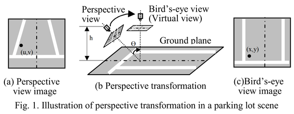
To obtain the output bird-s eye view image a transformation using the following projection matrix can be used. It maps the relationship between pixel (x,y) of the bird's eye view image and pixel (u,v) from the input image.
[math]\displaystyle{ \begin{bmatrix} x'\\ y'\\ w' \end{bmatrix} = \begin{bmatrix} a_{11} & a_{12} & a_{13}\\ a_{21} & a_{22} & a_{23}\\ a_{31} & a_{32} & a_{33} \end{bmatrix} \begin{bmatrix} u\\ v\\ w \end{bmatrix} \;\; where \;\;\;\; x = \frac{x'}{w'} \;\; and \;\;\;\; y = \frac{y'}{w'}. }[/math]
The transformation is usually referred to as Inverse Perspective Mapping (IPM) [3]. IPM takes as input the frontal view, applies a homography, and creates a top-down view of the captured scene by mapping pixels to a 2D frame (Bird's eye view).
In practice, IPM works great in the immediate proximity of a car, for example, and assuming the road surface is planar. Geometric properties of objects in the distance are affected unnaturally by this non-homogeneous mapping, as shown in Figure 2 left image. This limits the performance of applications in terms of accuracy and distance where they can be applied reliably. The right image can be achieved by applying several post-transformation techniques like Incremental Spatial Transformer [4]. However, this project uses a basic IPM approach as a demonstration.
There are 3 assumptions when working without post-transformation techniques:
- The camera is in a fixed position with respect to the road.
- The road surface is planar.
- The road surface is free of obstacles.
Camera Model and Homography
From the point of view of geometriacal characteristics, a pin-hole camera is a device that transforms a 3D world coordinate into a 2D image coordinate. This relation is described by the homography equation [5]:
[math]\displaystyle{ [u,v,1]^t \simeq P_{3x4} \cdot [X,Y,Z,1]^t \;\;\;\;\;\; (1) }[/math]
Matrix is decomposed into:
[math]\displaystyle{ P_{3x4} = K_{3x3} \cdot [R_{3x3}|t_{3x1}] \;\;\;\;\;\; (2) }[/math]
Where [math]\displaystyle{ R_{3x3} }[/math] is a 3x3 rotation matrix, [math]\displaystyle{ t_{3x1} }[/math] is a 3x1 translation vector, and [math]\displaystyle{ [R_{3x3}|t_{3x1}] }[/math] is a 3x4 matrix reflecting the concatenation of previous two, which handles the camera position and angles relative to the 3D world coordinate frame.
The homogeneous 3D coordinate of the point on the plane is described by (3), where [math]\displaystyle{ Q }[/math] is a 4x3 matrix.
[math]\displaystyle{ [X,Y,Z,1]^t = \begin{bmatrix} x \cdot i + y \cdot j + d \\ 1 \end{bmatrix} = Q_{4x3} \cdot [x,y,1]^t \;\;\;\;\;\; (3) }[/math]
By substituting (3) for (1), (4) is obtained which indicates the relation between the 2D coordinates of a plane in the scene and the image plane is described by a 3x3 matrix H in the homogeneous sense.
[math]\displaystyle{ [u,v,1]^t \simeq P_{3x4} \cdot Q_{4x3} \cdot [x,y,1]^t = H_{3x3} \cdot [x,y,1]^t \;\;\;\;\;\; (4) }[/math]
RidgeRun BEV Demo Workflow
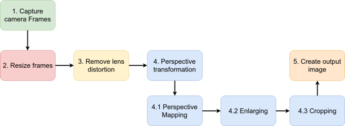
The following image shows the basic processing path used by the BEV system.
- Capture camera frames: Obtain frames from a video source. 4 cameras with 180 degrees view angle.
- Resize frames: Resize input frames to desired input size.
- Remove lens distortion: Apply lens undistortion algorithm to remove the fisheye effect.
- Perspective transformation: Use the IPM
- Perspective mapping: Map the points from the front view image to a 2D top image (BEV)
- Enlarging: Enlarge the image to search for the required region of interest (ROI)
- Cropping: Crop the output of the enlargement process to adjust the needed view.
- Create a final top view image
Removing fisheye distortion
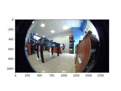
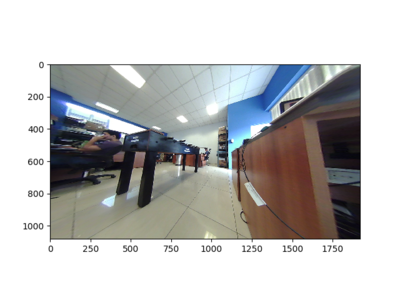
Wide-angle cameras are needed to obtain the max point of view and to achieve the Bird's Eye View perspective. Usually, these cameras provide fish eye image which needs to be transformed to remove the distortion. After the camera calibration process was done, done parameters are received:
- K: Output 3x3 floating-point camera matrix
[math]\displaystyle{ K= \begin{bmatrix} f_{x} & 0 & c_{x}\\ 0 & f_{y} & c_{y}\\ 0 & 0 & 1 \end{bmatrix} }[/math]
- D: Output vector of distortion coefficients
[math]\displaystyle{ D = [K_{1},K_{2},K_{3},K_{4}] }[/math]
As stated in the OpenCV documentation, let P be a point in 3D of coordinates X in the world reference frame (stored in the matrix X) The coordinate vector of P in the camera reference frame is
[math]\displaystyle{ Xc = R X + T }[/math]
where R is the rotation matrix corresponding to the rotation vector om: R = rodrigues(om); call x, y and z the 3 coordinates of Xc:
[math]\displaystyle{ x = Xc_{1}, \;\; y = Xc_{2}, \;\; z = Xc_{3} }[/math]
The pinhole projection coordinates of P is [a; b] where
[math]\displaystyle{ a = \frac{x}{z}, \;\; b = \frac{y}{z}, \;\; r^2 = a^2 + b^2, \;\; \theta = a \; tan(r) }[/math]
The fisheye distortion is defined by:
[math]\displaystyle{ \theta_{d} = \theta(1+k_{1}\theta^2+k_{2}\theta^4+k_{3}\theta^6+k_{4}\theta^8) }[/math]
The distorted point coordinates are [x'; y'] where
[math]\displaystyle{ x' = (\theta_{d} / r ) a , \;\; y' = (\theta_{d} / r ) b }[/math]
Perspective Mapping
The first step is to apply the perspective mapping from the input image to transform the angle image into a top view. Then, the enlarge process allows matching the output image perspective and the crop step handles to capture the required region of interest, as seen in the following image.
Process Optimization
The process described so far is based on state-of-the-art papers and research on how to apply IPM and other techniques to generate a top view image. The minimal steps always include the perspective mapping to get the IPM result, enlargement to adjust the measures between different cameras, and cropping to use only the required part of the image. These steps work great for a single image in an isolated environment to analyze and generate a single output frame. However, when the process needs to be repeated once for each frame at higher frame rates the system stress might be too high, and therefore the frame rate might be lower than expected.
To enhance the performance of the library we designed a simple method to wrap up all of the steps in a single warp perspective method. Usually, in Computer Vision, two images of the same planar surface in space can be related by a homography matrix. The method has many practical applications like image rectification, image registration, or computation of camera motion rotation, resize, and translation between two images. We will rely on the last application to speed up the process.
[math]\displaystyle{ H = \begin{bmatrix} h_{00} & h_{01} & h_{02}\\ h_{10} & h_{11} & h_{12}\\ h_{20} & h_{21} & h_{22} \end{bmatrix} }[/math]
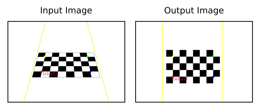
From an input image we need to map each [math]\displaystyle{ x_1,y_1 }[/math] source point to another [math]\displaystyle{ x_2,y_2 }[/math] destination point. The library uses a chessboard to collect inner corners and automatically adjust them by generating a perfect squared relationship and generate the output image as seen in the following figure.
The relationship between the points is defined by:
[math]\displaystyle{ \begin{bmatrix} x_{1} \\ y_{1} \\ 1 \end{bmatrix} = H \cdot \begin{bmatrix} x_{2} \\ y_{2} \\ 1 \end{bmatrix} = \begin{bmatrix} h_{00} & h_{01} & h_{02}\\ h_{10} & h_{11} & h_{12}\\ h_{20} & h_{21} & h_{22} \end{bmatrix} \begin{bmatrix} x_{2} \\ y_{2} \\ 1 \end{bmatrix} }[/math]
The main objective is to focus on how to adjust the homography matrix to absorb all the previous steps. With several geometric transformation the library also allows the user to fine-tune the final image. Matrix multiplication allows the quick and easy modification of the final homography, therefore the operation will be defined by [math]\displaystyle{ T_1 }[/math] (Move image to origin), [math]\displaystyle{ S_1 }[/math] (Scale image), [math]\displaystyle{ T_2 }[/math] (Move image back to original position), [math]\displaystyle{ M_1 }[/math] (Move image to fine adjust position), [math]\displaystyle{ A_1 }[/math] (Rotate image). The final homography ([math]\displaystyle{ H_f }[/math]) will be defined by:
[math]\displaystyle{ H_f = H \cdot T_1 \cdot S_1 \cdot T_2 \cdot M_1 \cdot A_1 }[/math]
where [math]\displaystyle{ T_1 }[/math], [math]\displaystyle{ S_1 }[/math], [math]\displaystyle{ T_2 }[/math] , [math]\displaystyle{ M_1 }[/math], [math]\displaystyle{ A_1 }[/math] are:
[math]\displaystyle{ T_1 = \begin{bmatrix} 0 & 1 & -centerX\\ 0 & 1 & -centerY\\ 0 & 0 & 1\\ \end{bmatrix} \;\; S_1 = \begin{bmatrix} scaleX & 0 & 0\\ 0 & scaleY & 0\\ 0 & 0 & 1\\ \end{bmatrix} \;\; T_2 = \begin{bmatrix} 0 & 1 & centerX\\ 0 & 1 & centerY\\ 0 & 0 & 1\\ \end{bmatrix} \;\; M_1 = \begin{bmatrix} 1 & 0 & moveX\\ 0 & 1 & moveY\\ 0 & 0 & 1\\ \end{bmatrix} \;\; A_1 = \begin{bmatrix} cos(angle) & -sin(angle) & 0\\ sin(angle) & -cos(angle) & 0\\ 0 & 0 & 1\\ \end{bmatrix} }[/math]
The input parameters for each matrix are:
- CenterX: Calculated X center between the inner corners of the chessboard
- CenterY: Calculated Y center between the inner corners of the chessboard
- ScaleX, ScaleY: User defined scale factor for the output image
- MoveX, MoveY: User defined amount of image movement adjustment
- Angle: User defined rotation angle
