Full Body Pose Estimation for Sports Analysis - Temporal Filter
WORK IN PROGRESS. Please Contact RidgeRun OR email to support@ridgerun.com if you have any questions. |
Introduction
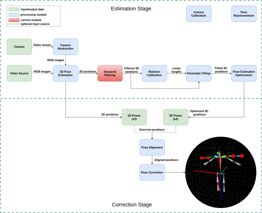
The temporal filter module is intended to reduce the noise from the 3D pose estimation process. This filter uses adaptive control to adjust to different movement speeds, which will provide a better frame sequence reconstruction.
Filter Description
The temporal filter is a low pass filter described by the equation:
[math]\displaystyle{ y[n] = \beta y[n-1] + (1 - \beta)x[n]; \;\;\;\;\;\; n = 0,1,2,3 \dots \;\;\;\;\;\; (1) }[/math]
where
- [math]\displaystyle{ y[n-1] }[/math] is the last filtered sample.
- [math]\displaystyle{ x[n] }[/math] is the sample to filter.
- [math]\displaystyle{ \beta }[/math] is a parameter between 0 and 1 to control how much of the input sample is filtered. If the value is close to 0 the sample will be barely filtered, and if it is close to 1, the filtered sample will be very similar to the last filtered sample.
In this case it is assumed that [math]\displaystyle{ y[0] = x[0] }[/math].
Adaptation
The control parameter [math]\displaystyle{ \beta }[/math] may be either fixed or adaptive, as it is in this case. The adaptation process is computed after every new sample is filtered, and the equation that describes the process is:
[math]\displaystyle{ \beta = 1 - \gamma^m \;\;\;\;\;\; (2) }[/math]
where
- [math]\displaystyle{ \gamma }[/math] is a number between 0 and 1 that defines the minimum value that [math]\displaystyle{ \beta }[/math] may take.
- [math]\displaystyle{ m }[/math] is a constantly changing parameter according to the following conditions:
- If the difference between the last filtered sample and its original non-filtered version is greater than a threshold [math]\displaystyle{ \epsilon }[/math], then [math]\displaystyle{ m }[/math] decreases, causing that [math]\displaystyle{ \beta }[/math] decreases too. The lower limit of this parameter is 1, which will give the lowest possible value to [math]\displaystyle{ \beta }[/math].
- If the difference between the last filtered sample and its original non-filtered version is equal or lower than a threshold [math]\displaystyle{ \epsilon }[/math], then [math]\displaystyle{ m }[/math] increases, causing that [math]\displaystyle{ \beta }[/math] increases too. The upper limit of this parameter is customizable, but keep in mind that the higher the limit, the harder it will be later to decrease it to its minimum.
It is possible to define different movement thresholds [math]\displaystyle{ \epsilon }[/math] for each type of data contained in the sample.
Example
In this example, the filter was used to remove the noise from a 3D pose estimation process. Some considerations taken in the process are:
- There was a different movement threshold for each skeleton joint.
- The [math]\displaystyle{ \gamma }[/math] parameter had a value of 0.9.
- The upper limit for [math]\displaystyle{ m }[/math] was 30.
In Figure 2 we present an example of how the filter works, by showing the raw input in the upper image and the filtered output in the image below. In this animation, you may notice that some of the limbs of the upper skeleton are constantly jumping, for example, the shoulders. Meanwhile, in the skeleton below, this movement is smoothed by our filter without losing the movement's intention.
Also, the [math]\displaystyle{ \beta }[/math] parameter behavior can be seen in Figure 3. Here it is visible that the parameter constantly changes according to movement speed in the video above.
How to Use the Module
Here we will explain how the filtering of the example above was developed in order to have a better understanding of the module usage. If you want to see an example of how to use the filter with skeleton visualization, check the How to Use the Library section.
- First, import the temporal filter module from the pose estimation library.
from pose_estimation.filter.temporal_filtering import *
- Next step is to define the threshold values for the positions that will be filtered. These threshold values define when it is considered that an object has moved a lot, so you should experiment with different values to see which ones suit each object better.
In our example, we have 15 joint positions, which means that we must provide a threshold for each of them.
 #Thresholds in cm
 JOINTS_THRESHOLDS = [5, 10, 0, 7, 3, 5, 20, 3, 5, 7, 3, 5, 20, 3, 5]
- Now we have to define the filter parameters explained above. As it was mentioned, the gamma and m parameters will define the beta parameter behavior, which is how much effect will have the filter.
In this example we want to allow quick and slow movements, which means that our beta parameters need to have a wide range of values. By using [math]\displaystyle{ \gamma = 0.9 }[/math] and limiting [math]\displaystyle{ m }[/math] to 30 our betas would have a range of [0.1, 0.96].
 #Filter parameters
 GAMMA = 0.9
 M_LIMIT = 30
- Now we can initialize our filter object.
filter = TemporalFilter(JOINTS_THRESHOLDS, GAMMA, M_LIMIT)
- Next step is to start filtering. Let's say that we have an array of joint positions that were taken on a sequence of frames, then each frame has a set of 15 3D positions. We will be storing the filtered positions in a new array to use them later.
 filtered_frame_positions_array = numpy.array(0,15,3)
 for frame_positions in frame_positions_array:
     #filter function
     filtered_positions = filter.filter_sample(frame_positions)
     filtered_frame_positions_array = numpy.append(filtered_frame_positions_array, filtered_positions)
- Finally, we can visually analyze the behavior of the beta parameter adaptation during the filtering process. We should provide the number of rows and columns in which the plots will be organized.
Here we have 15 joints, so a grid of 3 rows and 5 columns will be enough.
filter.plot_betas(3,5)


